The purpose of this analysis is to create a quick and dirty forecast of the CCI30 Crypto Currency Index, using only a few lines of R code and easy-to-use and accurate time series forecasting models.
The CCI30 Crypto Currency Index https://cci30.com/ “…is a rules-based index designed to objectively measure the overall growth, daily and long-term movement of the blockchain sector. It does so by tracking the 30 largest cryptocurrencies by market capitalization. It serves as a tool for passive investors to participate in this asset class, and as an industry benchmark for investment managers.“
The CCI30 is a product of Igor Rivin and Carlo Scevola.

Package Dependencies for Forecasts
So it’s time for a short review and forecast. To do this, I use R inside of RStudio. I use the following packages with this quick piece of code:
install.load::install_load(
  "tidyquant"
  ,"timetk"
  , "tibbletime"
  , "sweep"
  , "anomalize"
  , "caret"
  , "forecast"
  , "funModeling"
  , "xts"
  , "fpp"
  , "lubridate"
  , "tidyverse"
  , "urca"
  , "prophet"
)
The Data
From the CCI30 (who graciously make their index data available), I grab the file, and we have the Date and OHLCV (Open, High, Low, Close, Volume) columns. We can inspect the first row of the data:
head(df.tibble, 1)
# A time tibble: 1 x 6
# Index: Date
  Date        Open  High   Low Close       Volume

1 2019-12-30 2546. 2578. 2481. 2501. 45315440388.
Data Wrangling and Exploratory Analysis
A simple feature plot of the OHLCV gives the following:

From there I generate the daily return and log daily return of the closing price of the index. I then collapse the data by month and get the monthly log return.
df.ts.monthly <- df.ts.tbl %>%
  tq_transmute(
    select = Close
    , periodReturn
    , period = "monthly"
    , type = "log"
    , col_rename = "Monthly.Log.Returns"
    )
head(df.ts.monthly, 5)
# A time tibble: 5 x 2
# Index: Date
  Date       Monthly.Log.Returns

1 2015-01-31             -0.396
2 2015-02-28              0.0807
3 2015-03-31             -0.138
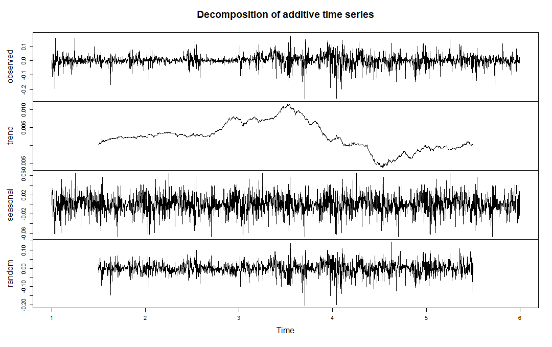
Here is a decomposition of the daily log return of the index:
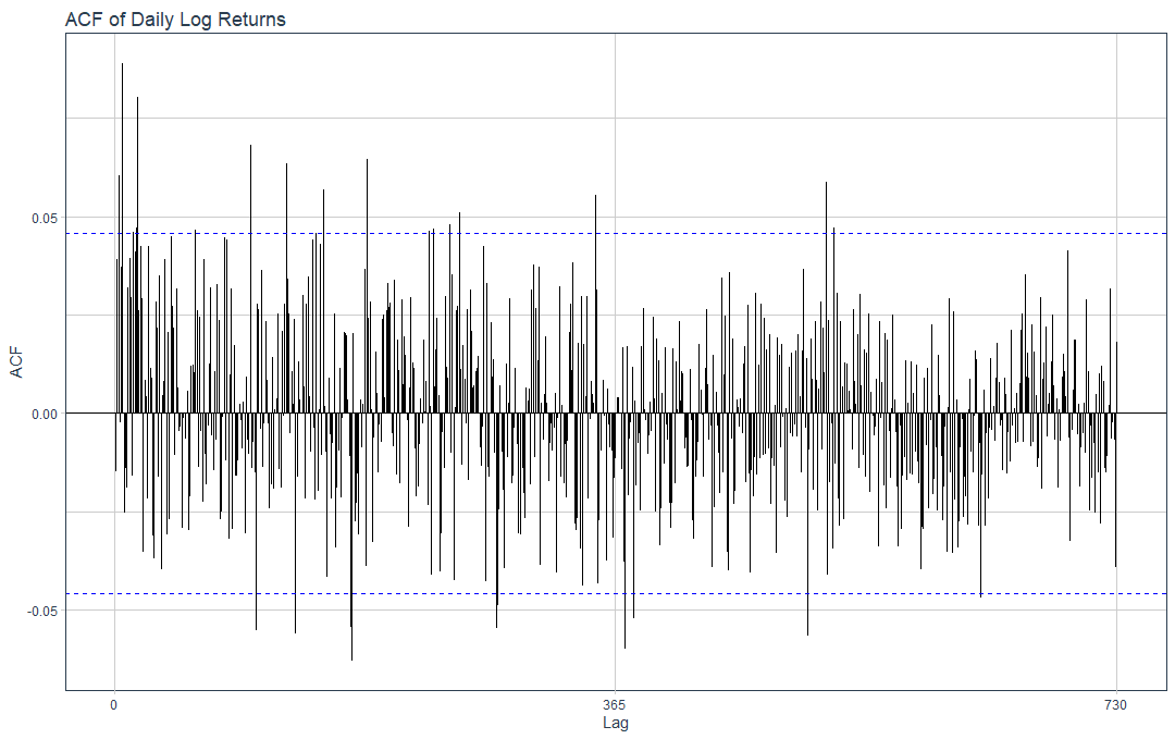
ACF (Auto Correlation Function) of Daily Log Returns:
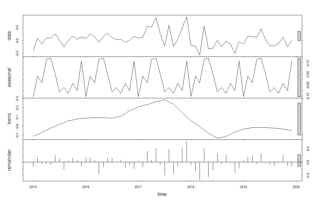
After collapsing the data into a monthly time series format we again take a look at the decomposition:
Anomaly Detection
Now, let us look for anomalies in the monthly data. To do this, I use the anomalize package.
dfa_tsb <- df.ts.monthly %>%
  time_decompose(Monthly.Log.Returns, method = "tiwtter") %>%
  anomalize(remainder, method = "gesd") %>%
  time_recompose()
dfa_tsb %>%
  plot_anomaly_decomposition() +
  xlab("Monthly Log Return") +
  ylab("Value") +
  labs(
    title = "Anomaly Detection for CCI30 Monthly Log Returns"
    , subtitle = "Method: GESD"
  )
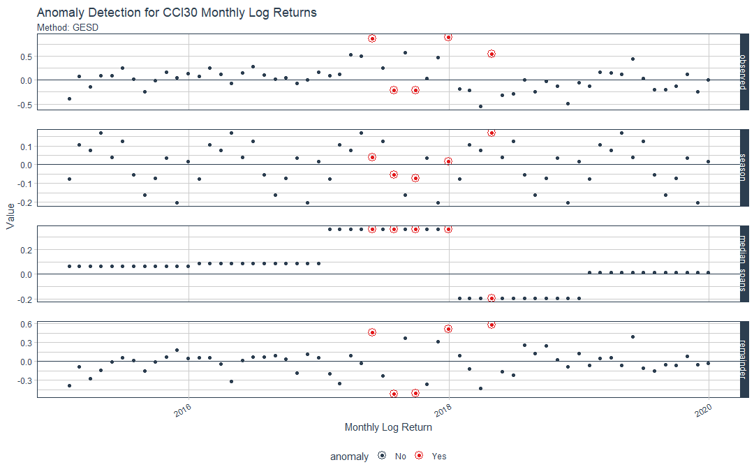
We can easily see the anomalous returns during, what I refer to as, the mainstream crypto craze of 2017.
CCI30 Index Forecasts
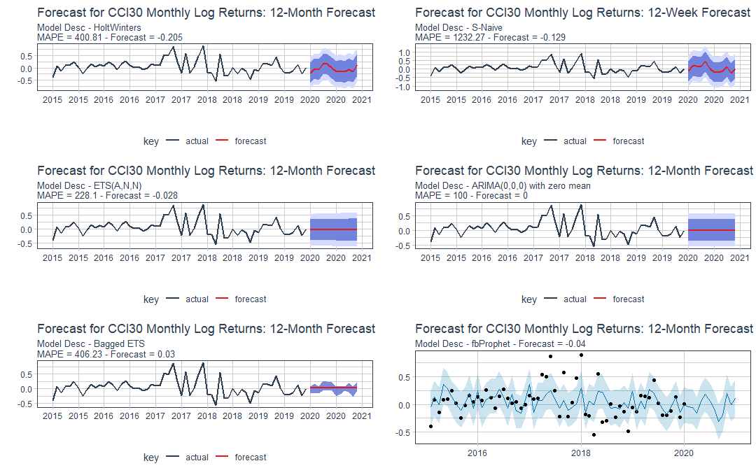
With all of this done, we move onto the forecast of the index. I forecast 12 months out using a few different models: HW (Holt-Winters), ETS (Error, Trend, Seasonality), Bagged ETS, ARIMA, SNaive and Facebook Prophet. These models produce the following:
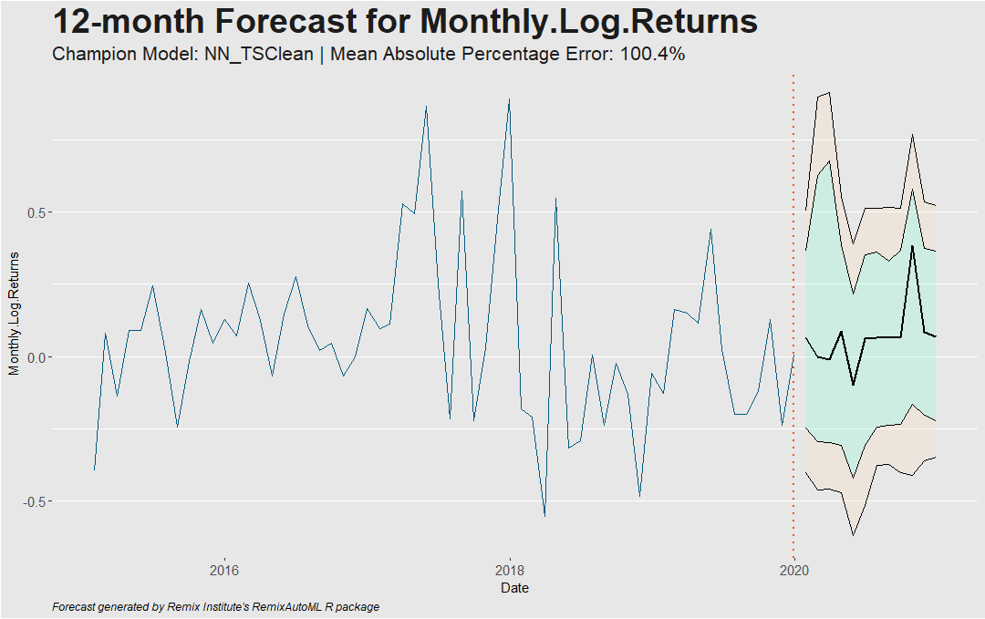
Automated Forecasting of CCI30 Using RemixAutoML
There is another package out called RemixAutoML where they provide an AutoTS (automated time series) function which we will also use and see if results differ.
You can find my code on my GitHub. Feel free to contribute to the project.
Steven Paul Sanderson II, MPH is a Data Scientist at Long Island Community Hospital. He has several years experience working in data science and analytics and holds a Master’s in Public Health from the Stony Brook University Health Sciences Center College of Medicine and a Bachelor’s in Economics from the State University of New York at Stony Brook. You can connect with him on LinkedIn at: https://www.linkedin.com/in/spsanderson/
